For Which Of The Following Goods Is Supply The Most Responsive To A Change In Price?

vii.2 Utility Maximization and Demand

Learning Objectives

1. Derive an individual demand bend from utility-maximizing adjustments to changes in price.
2. Derive the market demand curve from the demand curves of individuals.
3. Explain the exchange and income effects of a cost modify.
4. Explain the concepts of normal and inferior goods in terms of the income effect.

Choices that maximize utility—that is, choices that follow the marginal decision dominion—generally produce downward-sloping need curves. This department shows how an private's utility-maximizing choices can lead to a demand curve.

Deriving an Individual's Demand Curve

Suppose, for simplicity, that Mary Andrews consumes only apples, denoted by the letter of the alphabet A, and oranges, denoted by the letter of the alphabet O. Apples price $2 per pound and oranges cost $1 per pound, and her upkeep allows her to spend $20 per month on the ii appurtenances. We assume that Ms. Andrews will adjust her consumption so that the utility-maximizing condition holds for the two goods: The ratio of marginal utility to price is the aforementioned for apples and oranges. That is,

Equation 7.4

[latex]\frac{MU_A}{ \$ 2} = \frac{MU_O}{ \$ one}[/latex]

Here MU _A and MU _O are the marginal utilities of apples and oranges, respectively. Her spending equals her budget of $twenty per month; suppose she buys five pounds of apples and 10 of oranges.

At present suppose that an unusually big harvest of apples lowers their price to $one per pound. The lower toll of apples increases the marginal utility of each $1 Ms. Andrews spends on apples, so that at her current level of consumption of apples and oranges

Equation 7.5

[latex]\frac{MU_A}{ \$ 1} > \frac{MU_O}{ \$ one}[/latex]

Ms. Andrews will answer past purchasing more apples. As she does and so, the marginal utility she receives from apples will decline. If she regards apples and oranges as substitutes, she will also buy fewer oranges. That will cause the marginal utility of oranges to rising. She volition keep to adjust her spending until the marginal utility per $ane spent is equal for both goods:

Equation seven.half-dozen

[latex]\frac{MU_A}{ \$ 1} = \frac{MU_O}{ \$ 1}[/latex]

Suppose that at this new solution, she purchases 12 pounds of apples and eight pounds of oranges. She is still spending all of her budget of $20 on the two appurtenances [(12 x $one)+(8 x $1)=$20].

Figure vii.3 Utility Maximization and an Individual'south Demand Curve

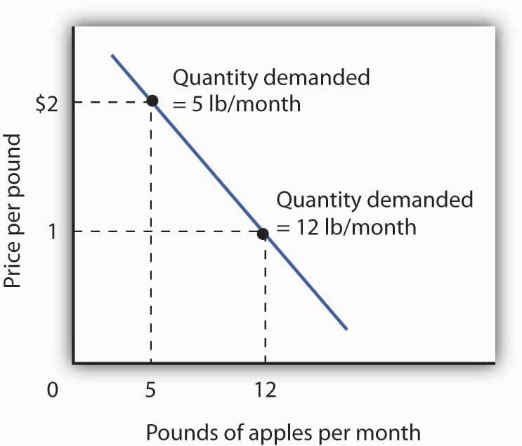
Mary Andrews's demand curve for apples, d, can be derived by determining the quantities of apples she will buy at each toll. Those quantities are determined by the application of the marginal decision rule to utility maximization. At a price of $2 per pound, Ms. Andrews maximizes utility by purchasing 5 pounds of apples per month. When the price of apples falls to $1 per pound, the quantity of apples at which she maximizes utility increases to 12 pounds per month.

Information technology is through a consumer'south reaction to different prices that we trace the consumer's demand curve for a good. When the cost of apples was $2 per pound, Ms. Andrews maximized her utility by purchasing 5 pounds of apples, as illustrated in Figure 7.3 "Utility Maximization and an Individual'due south Need Curve". When the price of apples brutal, she increased the quantity of apples she purchased to 12 pounds.

Heads Upwards!

Find that, in this instance, Ms. Andrews maximizes utility where not only the ratios of marginal utilities to price are equal, only also the marginal utilities of both goods are equal. But, the equal-marginal-utility event is merely true hither because the prices of the two goods are the aforementioned: each good is priced at $ane in this instance. If the prices of apples and oranges were dissimilar, the marginal utilities at the utility maximizing solution would have been different. The status for maximizing utility—consume where the ratios of marginal utility to price are equal—holds regardless. The utility-maximizing condition is not that consumers maximize utility by equating marginal utilities.

Utility maximizing condition is: [latex]\frac{MU_{X}}{P_{X}} = \frac{MU_{X}}{P_{Y}}[/latex]

Utility maximizing condition is not: [latex]MU_{X} = MU_{Y}[/latex]

From Individual to Market Demand

The market demand curves nosotros studied in previous chapters are derived from private need curves such as the 1 depicted in Figure 7.3 "Utility Maximization and an Private's Demand Curve". Suppose that in addition to Ms. Andrews, at that place are ii other consumers in the market place for apples—Ellen Smith and Koy Keino. The quantities each consumes at various prices are given in Figure 7.v "Deriving a Market Demand Curve", forth with the quantities that Ms. Andrews consumes at each cost. The demand curves for each are shown in Panel (a). The market demand curve for all three consumers, shown in Panel (b), is then establish by calculation the quantities demanded at each price for all three consumers. At a price of $2 per pound, for case, Ms. Andrews demands 5 pounds of apples per calendar month, Ms. Smith demands iii pounds, and Mr. Keino demands eight pounds. A total of 16 pounds of apples are demanded per month at this price. Adding the individual quantities demanded at $ane per pound yields market demand of twoscore pounds per month. This method of adding amounts forth the horizontal centrality of a graph is referred to every bit summing horizontally. The market demand curve is thus the horizontal summation of all the individual demand curves.

Figure 7.v Deriving a Market Demand Curve

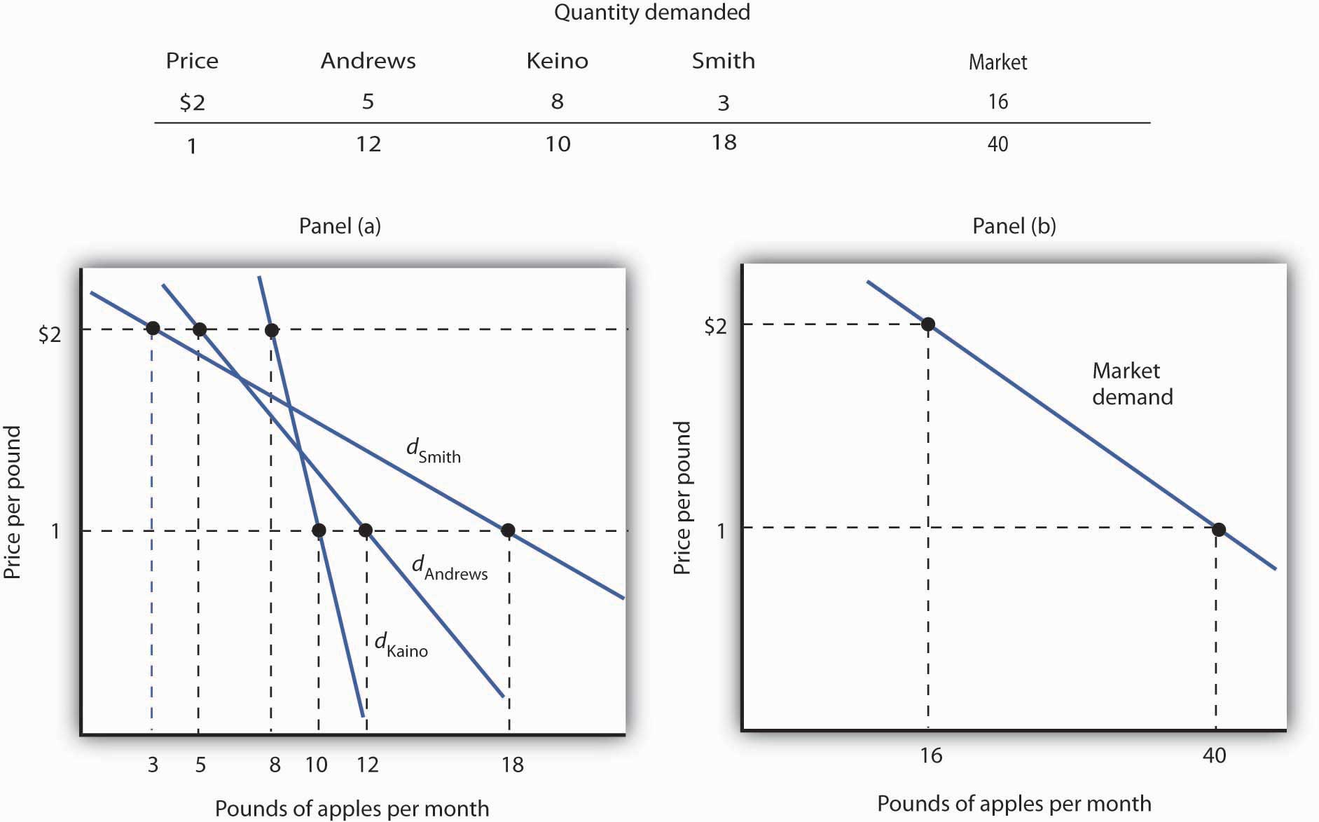
The need schedules for Mary Andrews, Ellen Smith, and Koy Keino are given in the table. Their individual demand curves are plotted in Panel (a). The market demand curve for all three is shown in Console (b).

Individual demand curves, then, reflect utility-maximizing adjustment by consumers to diverse market prices. Once more, we see that as the toll falls, consumers tend to buy more of a practiced. Demand curves are downwardly-sloping as the law of demand asserts.

Commutation and Income Effects

We saw that when the price of apples roughshod from $two to $one per pound, Mary Andrews increased the quantity of apples she demanded. Behind that adjustment, however, lie two distinct furnishings: the commutation effect and the income effect. It is important to distinguish these effects, because they can have quite different implications for the elasticity of the demand curve.

First, the reduction in the cost of apples made them cheaper relative to oranges. Before the price change, it price the same amount to buy two pounds of oranges or ane pound of apples. After the price change, it cost the same amount to purchase i pound of either oranges or apples. In effect, 2 pounds of oranges would exchange for 1 pound of apples before the price alter, and one pound of oranges would exchange for ane pound of apples after the price change.

Second, the cost reduction essentially made consumers of apples richer. Before the cost change, Ms. Andrews was purchasing 5 pounds of apples and 10 pounds of oranges at a total cost to her of $xx. At the new lower toll of apples, she could purchase this same combination for $15. In effect, the toll reduction for apples was equivalent to handing her a $five bill, thereby increasing her purchasing power. Purchasing ability refers to the quantity of goods and services that can be purchased with a given budget.

To distinguish between the substitution and income effects, economists consider starting time the impact of a cost change with no change in the consumer'southward ability to purchase goods and services. An income-compensated toll changeAn imaginary exercise in which we assume that when the price of a practiced or service changes, the consumers income is adjusted then that he or she has just enough to purchase the original combination of goods and services at the new set of prices. is an imaginary exercise in which we assume that when the price of a good or service changes, the consumer's income is adjusted then that he or she has just enough to purchase the original combination of goods and services at the new set of prices. Ms. Andrews was purchasing five pounds of apples and 10 pounds of oranges before the price change. Buying that same combination later on the cost change would cost $15. The income-compensated price change thus requires united states of america to take $5 from Ms. Andrews when the toll of apples falls to $one per pound. She tin can still purchase 5 pounds of apples and ten pounds of oranges. If, instead, the price of apples increased, we would give Ms. Andrews more money (i.due east., we would "recoup" her) and then that she could purchase the aforementioned combination of goods.

With $15 and cheaper apples, Ms. Andrews could buy five pounds of apples and 10 pounds of oranges. Merely would she? The reply lies in comparison the marginal do good of spending some other $1 on apples to the marginal benefit of spending another $1 on oranges, as expressed in Equation 7.5. It shows that the actress utility per $1 she could obtain from apples now exceeds the extra utility per $1 from oranges. She volition thus increase her consumption of apples. If she had merely $15, any increase in her consumption of apples would crave a reduction in her consumption of oranges. In effect, she responds to the income-compensated price change for apples past substituting apples for oranges. The change in a consumer's consumption of a proficient in response to an income-compensated price change is called the exchange consequenceThe change in a consumers consumption of a expert in response to an income-compensated price alter. .

Suppose that with an income-compensated reduction in the price of apples to $1 per pound, Ms. Andrews would increase her consumption of apples to 9 pounds per month and reduce her consumption of oranges to 6 pounds per calendar month. The exchange effect of the price reduction is an increase in apple consumption of 4 pounds per calendar month.

The commutation result ever involves a change in consumption in a management reverse that of the price change. When a consumer is maximizing utility, the ratio of marginal utility to price is the same for all goods. An income-compensated price reduction increases the extra utility per dollar available from the good whose toll has fallen; a consumer volition thus purchase more of it. An income-compensated price increase reduces the extra utility per dollar from the good; the consumer volition purchase less of information technology.

In other words, when the price of a good falls, people react to the lower toll by substituting or switching toward that adept, buying more than of it and less of other appurtenances, if nosotros artificially hold the consumer's power to buy goods constant. When the price of a skilful goes up, people react to the higher cost past substituting or switching abroad from that good, buying less of it and instead buying more than of other goods. Past examining the impact of consumer purchases of an income-compensated toll change, nosotros are looking at just the change in relative prices of goods and eliminating any impact on consumer buying that comes from the constructive change in the consumer's ability to purchase goods and services (that is, we hold the consumer'southward purchasing power abiding).

To consummate our analysis of the impact of the toll change, nosotros must now consider the $5 that Ms. Andrews effectively gained from it. Afterwards the cost reduction, it cost her just $fifteen to buy what cost her $20 before. She has, in effect, $5 more than she did before. Her additional income may also have an outcome on the number of apples she consumes. The change in consumption of a good resulting from the implicit change in income because of a price change is called the income effectThe change in consumption of a practiced resulting from the implicit change in income considering of a price alter. of a toll alter. When the cost of a good rises, at that place is an implicit reduction in income. When the price of a good falls, in that location is an implicit increment. When the price of apples fell, Ms. Andrews (who was consuming 5 pounds of apples per month) received an implicit increase in income of $5.

Suppose Ms. Andrews uses her implicit increase in income to purchase iii more pounds of apples and 2 more pounds of oranges per calendar month. She has already increased her apple consumption to 9 pounds per month considering of the substitution effect, then the added three pounds brings her consumption level to 12 pounds per month. That is precisely what we observed when we derived her demand curve; it is the modify nosotros would find in the marketplace. We see at present, nevertheless, that her increase in quantity demanded consists of a substitution consequence and an income effect. Figure 7.6 "The Substitution and Income Effects of a Price Change" shows the combined effects of the price change.

Figure 7.6 The Substitution and Income Effects of a Toll Alter

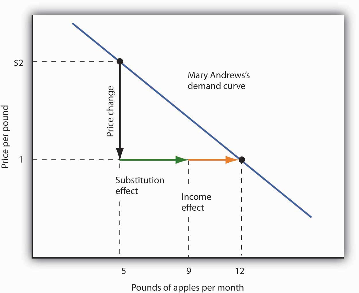
This demand curve for Ms. Andrews was presented in Effigy 7.5 "Deriving a Marketplace Demand Curve". Information technology shows that a reduction in the toll of apples from $2 to $one per pound increases the quantity Ms. Andrews demands from 5 pounds of apples to 12. This graph shows that this change consists of a commutation effect and an income effect. The substitution effect increases the quantity demanded past 4 pounds, the income outcome by 3, for a total increase in quantity demanded of seven pounds.

The size of the substitution effect depends on the rate at which the marginal utilities of goods change as the consumer adjusts consumption to a price change. As Ms. Andrews buys more than apples and fewer oranges, the marginal utility of apples will fall and the marginal utility of oranges volition rise. If relatively small changes in quantities consumed produce large changes in marginal utilities, the substitution effect that is required to restore the equality of marginal-utility-to-price ratios will be small. If much larger changes in quantities consumed are needed to produce equivalent changes in marginal utilities, then the exchange result will be large.

The magnitude of the income effect of a cost change depends on how responsive the demand for a good is to a change in income and on how important the good is in a consumer'southward budget. When the toll changes for a proficient that makes up a substantial fraction of a consumer's upkeep, the modify in the consumer's ability to buy things is substantial. A change in the toll of a skilful that makes upwards a trivial fraction of a consumer'southward budget, still, has footling effect on his or her purchasing power; the income consequence of such a price change is small.

Because each consumer's response to a price change depends on the sizes of the substitution and income effects, these effects play a role in determining the toll elasticity of demand. All other things unchanged, the larger the substitution event, the greater the absolute value of the price elasticity of demand. When the income effect moves in the same direction as the substitution effect, a greater income effect contributes to a greater toll elasticity of demand equally well. There are, however, cases in which the exchange and income effects motion in opposite directions. Nosotros shall explore these ideas in the side by side section.

Normal and Junior Appurtenances

The nature of the income effect of a toll change depends on whether the good is normal or inferior. The income effect reinforces the exchange effect in the case of normal goods; it works in the opposite direction for inferior goods.

Normal Goods

A normal good is one whose consumption increases with an increase in income. When the cost of a normal skilful falls, there are two identifying effects:

1. The substitution effect contributes to an increase in the quantity demanded considering consumers substitute more of the good for other goods.
2. The reduction in cost increases the consumer'due south ability to purchase appurtenances. Because the proficient is normal, this increase in purchasing power further increases the quantity of the good demanded through the income effect.

In the case of a normal good, then, the substitution and income effects reinforce each other. Ms. Andrews's response to a price reduction for apples is a typical response to a lower cost for a normal good.

An increment in the price of a normal proficient works in an equivalent mode. The higher price causes consumers to substitute more than of other goods, whose prices are at present relatively lower. The substitution effect thus reduces the quantity demanded. The higher cost likewise reduces purchasing power, causing consumers to reduce consumption of the skilful via the income effect.

Junior Goods

In the chapter that introduced the model of demand and supply, nosotros saw that an junior skillful is one for which need falls when income rises. It is likely to be a practiced that people do not really like very much. When incomes are low, people swallow the junior good because it is what they can afford. As their incomes rising and they tin afford something they similar better, they consume less of the inferior good. When the price of an inferior skillful falls, two things happen:

1. Consumers will substitute more of the inferior practiced for other appurtenances because its toll has fallen relative to those appurtenances. The quantity demanded increases equally a result of the substitution effect.
2. The lower price finer makes consumers richer. But, because the expert is inferior, this reduces quantity demanded.

The case of inferior goods is thus quite dissimilar from that of normal goods. The income effect of a price alter works in a direction opposite to that of the commutation result in the example of an junior expert, whereas it reinforces the substitution upshot in the case of a normal good.

Figure seven.seven Substitution and Income Effects for Inferior Appurtenances

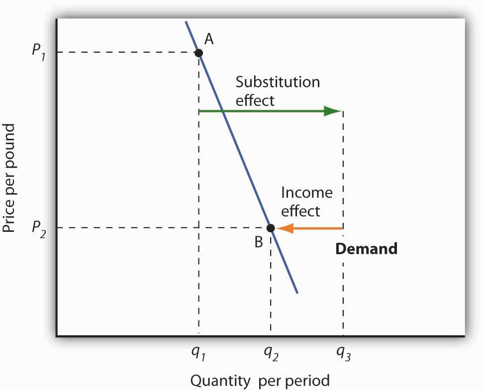
The substitution and income effects work against each other in the example of junior goods. The consumer begins at point A, consuming q ₁ units of the proficient at a cost P ₁. When the price falls to P _ii, the consumer moves to signal B, increasing quantity demanded to q _ii. The exchange effect increases quantity demanded to q _{due south}, but the income effect reduces it from q _southward to q ₂.

Figure 7.7 "Substitution and Income Effects for Junior Goods" illustrates the substitution and income effects of a price reduction for an inferior good. When the cost falls from P _one to P ₂, the quantity demanded by a consumer increases from q ₁ to q ₂. The commutation result increases quantity demanded from q _i to q _s. But the income issue reduces quantity demanded from q _s to q ₂; the substitution outcome is stronger than the income effect. The outcome is consistent with the police force of demand: A reduction in price increases the quantity demanded. The quantity demanded is smaller, nevertheless, than it would be if the skilful were normal. Junior appurtenances are therefore likely to have less rubberband demand than normal goods.

Key Takeaways

• Private demand curves reflect utility-maximizing adjustment by consumers to changes in price.
• Market place demand curves are found by summing horizontally the demand curves of all the consumers in the market.
• The substitution consequence of a cost change changes consumption in a management contrary to the price alter.
• The income upshot of a cost change reinforces the substitution outcome if the skillful is normal; information technology moves consumption in the opposite direction if the good is inferior.

Endeavor It!

Ilana Drakulic has an entertainment budget of $200 per semester, which she divides among purchasing CDs, going to concerts, eating in restaurants, and then along. When the price of CDs barbarous from $20 to $10, her purchases rose from 5 per semester to ten per semester. When asked how many she would have bought if her upkeep constraint were $150 (since with $150 she could continue to purchase v CDs and as before yet have $100 for spending on other items), she said she would accept bought 8 CDs. What is the size of her exchange effect? Her income effect? Are CDs normal or inferior for her? Which exhibit, Effigy 7.six "The Substitution and Income Effects of a Cost Change" or Figure 7.7 "Substitution and Income Effects for Inferior Goods", depicts more accurately her need curve for CDs?

Case in Indicate: Found! An Upward-Sloping Demand Curve

Figure 7.8

Charles Haynes – rice – CC BY-SA 2.0.

The fact that income and substitution effects move in opposite directions in the case of inferior goods raises a tantalizing possibility: What if the income effect were the stronger of the two? Could demand curves be upward sloping?

The answer, from a theoretical signal of view, is yep. If the income effect in Figure 7.vii "Substitution and Income Furnishings for Inferior Appurtenances" were larger than the commutation effect, the decrease in price would reduce the quantity demanded below q ₁. The upshot would be a reduction in quantity demanded in response to a reduction in cost. The demand curve would be upwardly sloping!

The suggestion that a good could take an upward-sloping demand curve is generally attributed to Robert Giffen, a British journalist who wrote widely on economic matters tardily in the nineteenth century. Such goods are thus called Giffen goods. To authorize equally a Giffen skillful, a good must exist junior and must have an income effect stiff plenty to overcome the substitution effect. The case often cited of a possible Giffen expert is the potato during the Irish famine of 1845–1849. Empirical analysis by economists using available data, yet, has refuted the notion of the upwards-sloping demand bend for potatoes at that fourth dimension. The most convincing parts of the refutation were to point out that (a) given the dearth, there were not more potatoes available for buy so and (b) the toll of potatoes may not have fifty-fifty increased during the menstruation!

A recent study by Robert Jensen and Nolan Miller, though, suggests the possible discovery of a pair of Giffen appurtenances. They began their search by thinking most the blazon of good that would be likely to showroom Giffen behavior and argued that, like potatoes for the poor Irish, it would exist a main dietary staple of a poor population. In such a situation, purchases of the detail are such a big percentage of the diet of the poor that when the particular's toll rises, the implicit income of the poor falls drastically. In order to subsist, the poor reduce consumption of other goods so they tin purchase more of the staple. In so doing, they are able to reach a caloric intake that is higher than what tin can exist achieved by ownership more of other preferred foods that unfortunately supply fewer calories.

Their preliminary empirical work shows that in southern Mainland china rice is a Giffen expert for poor consumers while in northern Communist china noodles are a Giffen proficient. In both cases, the basic practiced (rice or noodles) provides calories at a relatively low cost and dominates the diet, while meat is considered the tastier merely higher toll-per-calorie food. Using detailed household data, they estimate that among the poor in southern Mainland china a ten% increase in the price of rice leads to a x.4% increase in rice consumption. For wealthier households in the region, rice is inferior simply not Giffen. For both groups of households, the income effect of a price alter moves consumption in the opposite direction of the substitution effect. Simply in the poorest households, however, does it swamp the substitution effect, leading to an upwardly-sloping demand curve for rice for poor households. In northern China, the net outcome of a toll increase on quantity demanded of noodles is smaller, though it still leads to higher noodle consumption in the poorest households of that region.

In a similar study, David McKenzie tested whether tortillas were a Giffen good for poor Mexicans. He constitute, nevertheless, that they were an inferior expert but not a Giffen proficient. He speculated that the dissimilar result may stem from poor Mexicans having a wider range of substitutes available to them than do the poor in People's republic of china.

Because the Jensen/Miller report is the showtime vindication of the existence of a Giffen good despite a very long search, the authors have avoided rushing to publication of their results. Rather, they accept fabricated bachelor a preliminary version of the study reported on here while standing to refine their estimation.

Sources: Robert Jensen and Nolan Miller, "Giffen Behavior: Theory and Bear witness," KSG Faculty Enquiry Working Papers Series RWP02-014, 2002 available at ksghome.harvard.edu/~nmiller/giffen.html or http://ssrn.com/abstract=310863. At the authors' request we include the following note on the preliminary version: "Because we have received numerous requests for this paper, we are making this early draft available. The results presented in this version, while strongly suggestive of Giffen behavior, are preliminary. In the most future we await to acquire additional information that will allow the states to revise our estimation technique. In particular, monthly temperature, atmospheric precipitation, and other atmospheric condition data will enable united states to employ an instrumental variables approach to address the possibility that the observed variation in prices is not exogenous. Once available, the instrumental variables results volition be incorporated into time to come versions of the paper." ; David McKenzie, "Are Tortillas a Giffen Skilful in Mexico?" Economics Bulletin 15:1 (2002): 1–seven.

Reply to Try It! Problem

I hundred fifty dollars is the income that allows Ms. Drakulic to buy the aforementioned items as before, and thus tin be used to measure the substitution event. Looking just at the income-compensated price change (that is, belongings her to the same purchasing power as in the original relative price situation), we find that the substitution effect is 3 more than CDs (from 5 to 8). The CDs that she buys beyond viii constitute her income effect; it is two CDs. Because the income issue reinforces the substitution effect, CDs are a normal good for her and her demand curve is like to that shown in Figure 7.6 "The Substitution and Income Effects of a Price Change".

Source: https://open.lib.umn.edu/principleseconomics/chapter/7-2-utility-maximization-and-demand/

Posted by: graytimit1951.blogspot.com

Share this post